Suggest multiple active spaces

Example: the para-benzyne diradical

# Suppress PySCF warning...
import pyscf
pyscf.__config__.B3LYP_WITH_VWN5 = False

from pathlib import Path
from pyscf.gto import Mole
from pyscf.lib import logger
from asf import ASFDMRG
from asf.visualization import draw_pair_information
from asf.preselection import MP2NatorbPreselection, MP2PairinfoPreselection
from asf.scf import stable_scf
from asf.utility import pictures_Jmol, show_mos_grid

1. Define the molecule as a PySCF object

In the ASF package, molecular systems are represented as PySCF Mole objects. The first step is therefore to initialize the example molecule as follows:

mol = Mole(
    atom="pbenzyne.xyz",
    spin=0,
    charge=0,
    basis="def2-SVP",
    verbose=logger.NOTE,  # a less talkative option, to suppress printing of SCF iterations, etc.
).build()

2. Perform a UHF calculation

This is intentional even for singlet states, as a broken-symmetry solution helps with active space selection. The function stable_scf incorporates checks for convergence and stability of the solution. SCF calculations are restarted if an unconverged or unstable solution is encountered. The stability analysis often helps with nudging the orbitals towards a broken-symmetry solution, but it does not always work out.

mf = stable_scf(mol)

-> Initiating a UHF calculation.
converged SCF energy = -229.093693646044  <S^2> = 2.3862867e-10  2S+1 = 1
<class 'pyscf.scf.uhf.UHF'> wavefunction has an internal instability
-> Restarting SCF due to instability of previous solution.
-> Initiating SCF restart number 1.
SCF not converged.
SCF energy = -229.208902943573 after 50 cycles  <S^2> = 1.4200757  2S+1 = 2.5846282
<class 'pyscf.scf.uhf.UHF'> wavefunction is stable in the internal stability analysis
-> Calculation did not converge.
-> Switching to Newton solver.
-> Initiating SCF restart number 2.
converged SCF energy = -229.24037519866  <S^2> = 1.8354377  2S+1 = 2.8882089
<class 'pyscf.soscf.newton_ah.SecondOrderUHF'> wavefunction is stable in the internal stability analysis
-> The calculated SCF solution is converged and stable.

Side note: the ASF package contains wrapper that perfom some of the steps outlined below (semi-)automatically in one function:

• asf.wrapper.sized_space_from_mol - determines an optimal active space of given size starting from a Mole object,

• asf.wrapper.sized_space_from_scf - determines an optimal active space of given size starting from an SCF solution,

• asf.wrapper.find_from_mol - selects an active space based on a minimum entropy threshold starting from a Mole object, and

• asf.wrapper.find_from_scf - selects an active space based on a minimum entropy threshold starting from an SCF solution.

The find_from_... wrapper variants also support a limiting window for the active space size via min_norb and max_norb arguments.

3. Determine an initial active space

This step concerns the definition of a subset of the MO space in which the final active space should be determined. While not mandatory, such a preselection step is recommended for larger systems. The ASF package implements two procedures to select an initial space:

• asf.preselection.MP2PairinfoPreselection - based on pair information from Møller-Plesset perturbation theory

• asf.preselection.MP2NatorbPreselection - based on MP2 natural occupation numbers

Custom preselection approaches may be implemented by deriving from asf.asfbase.Preselection.

# If set to True, determine the initial active space using pair information derived from
# Moller-Plesset theory (more complicated procedure).
use_mp_pairinfo = True

if use_mp_pairinfo:
    pre = MP2PairinfoPreselection(mf)
    active_space_pt = pre.select()
# Otherwise, just use MP2 natural orbitals with a specific cutoff.
else:
    pre = MP2NatorbPreselection(mf, lower=0.02, upper=1.98)
    active_space_pt = pre.select()

print(active_space_pt)

ActiveSpace: 14 electrons in 14 orbitals
  active MO indices: [12, 14, 15, 16, 17, 18, 19, 20, 21, 22, 23, 24, 25, 27]

4. Run multi-reference single point calculation

ASFCI / ASFDMRG are two important low-level interface classes for the functionality of the ASF to perform single-point calculations. Here, a DMRG calculation is set up using the initial active space previously determined.

sf = ASFDMRG(
    mol=mol,
    nel=active_space_pt.nel,
    mo_list=active_space_pt.mo_list,
    mo_coeff=active_space_pt.mo_coeff,
    maxM=250,
)

At this point, the DMRG interface is initialized including the default calculation settings. For a more extensive control of the FCI solver settings both ASFDMRG and ASFCI accept the fcisolver_kwargs argument (see available keys for DMRG and CASCI). To start the single-point calculation, the calculate method must be called which is implemented by all of the ASF interfaces.

sf.calculate()

CASCI E = -229.353059217334  E(CI) = -33.6920950048242  S^2 = 0.0000000

5. Find active spaces

With the finished single-point calculation finished, the determination of viable active spaces is available. The active space search relies on metrics such as single-orbital entropies and pair information from the diagonal of the two-body cumulant. The ASF interfaces provide several methods to determine active spaces:

• find_many() determining multiple reasonable active spaces sorted by number of active electrons and number of active orbitals.

• find_one_sized() which yields one active space matching a given number of active orbitals and/or a given number of active electrons.

• find_one_entropy() which yields one active space that has a minimal single-orbital entropy above a threshold that can be changed by the user (recommended).

• find_one_generic() which also yields one active space, but requires the user to define the selection criteria.

This interactive example focuses on the usage of find_many(). See other tutorials for how find_one_sized or find_one_entropy can be employed. Internally, find_many() first determines a large number of candidate spaces (via unfiltered_pairinfo_spaces()) and then applies up to three selection criteria to select spaces most likely to converge to a reasonable solution.

active_spaces = sf.find_many()

The resulting output is a dictionary whereby each value is a list of active space suggestions matching the number of electrons and number of orbitals in the key. Each item in the suggestion list is a MOListInfo dataclass containing the list of MO indices and additional metrics used for the selection procedure. For example:

{
    (2, 2): [
        MOListInfo(
            mo_list=[19, 20],
            nel=2,
            minimal=False,
            pairinfo_sum=0.6640700019980257,
            max_increment=0.0150994051180795,
            min_decrement=0.9691123584300709,
            min_entropy=0.6783514316563286,
            min_edge_sum=0.34325572898426215,
        )
    ],
    ...
}

6. Inspect suggested active spaces

Molecular orbital indices

To get an overview of the suggested active spaces, we print active space groups (in (N, M) notation) and the associated MO index lists. Note that the indices refer to the MO coefficient matrix sf.mo_coeff (and therefore also active_space_pt.mo_coeff).

for nel, nmo in active_spaces.keys():
    for mo_info in active_spaces[(nel, nmo)]:
        print(f"({nel}, {nmo}): {mo_info.mo_list}")

(2, 2): [19, 20]
(4, 4): [17, 19, 20, 22]
(6, 6): [17, 18, 19, 20, 21, 22]
(8, 8): [16, 17, 18, 19, 20, 21, 22, 23]
(10, 10): [15, 16, 17, 18, 19, 20, 21, 22, 23, 25]
(10, 10): [14, 16, 17, 18, 19, 20, 21, 22, 23, 24]
(12, 12): [14, 15, 16, 17, 18, 19, 20, 21, 22, 23, 24, 25]

Molecular orbital visualization

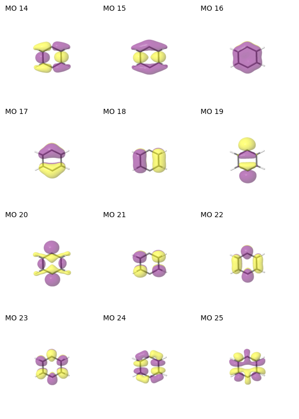
The suggested active MOs can be easily visualized by tools such as Jmol. The ASF package provides a utility function pictures_Jmol that creates a temporary molden file and writes the MO plots to the current working directory. To save a molden file for interactive inspection of the molecular orbitals, use:

from pyscf.tools import molden
molden.from_mo(mol, 'mos.molden', mo_coeff=sf.mo_coeff)

Once pictures_Jmol has run, there should be several images named mo_[index].png in the current directory. The function show_mos_grid from the utility module arranges the orbital images in a grid. The MO index lists seen in the previous step can also be passed to only show the MOs of the active space of interest. Note: MO indices in Jmol are indexed from one, not from zero. Thus, the annotation from Jmol is disabled and show_mos_grid annotates each orbital image with the MO index that is consistent with the ASF (0-indexed).

# If plots have been generated in a previous run of the Notebook, they will be reused here.
# Set redo_plots = True, if new orbital images should be created regardless of existing files.
redo_plots = False

# Select for which active space molecular orbitals should be shown:
space_of_interest = active_spaces[(12, 12)][0]

def mo_images(name_glob: str = "mo_*.png") -> list[Path]:
    """Return the list of all MO images in this directory."""
    return sorted(Path.cwd().glob(name_glob))

if redo_plots or not mo_images():
    pictures_Jmol(mol=mol, mo_coeff=sf.mo_coeff, mo_list=sf.mo_list, mo_index_title=" ")

show_mos_grid(mo_images(), mo_list=space_of_interest.mo_list, columns=3, figsize=(10, 10))

Pairinfo

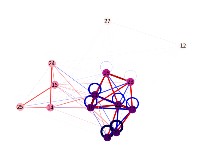
The ASF package also provides methods to visualize pair information which is a key metric in the active space search. Below, draw_pair_information() is employed to plot a graph of the pair information from the DMRG calculation. Note that the sign of the cumulant is inverted, so that the most energy-lowering interactions correspond to the largest pair information. In the resulting graph plot, the molecular orbitals are represented as nodes and the pair information as edges. Edges corresponding to energy-lowering interactions are colored red, while energy-raising interactions are shown in blue (cf. ‘seismic’ color map). By default the color of the nodes indicates the summed pair information per orbital using a sequential color map (‘RdPu’), however any per-orbital-quantity, such as single-orbital entropies, can be passed instead via the orbital_info argument.

pairinfo = -sf.diagonal_cumulant(full_space=False)
draw_pair_information(pair_info=pairinfo, orbital_labels=sf.mo_list)

      MO    orb. value
      12        0.0097
      14        0.0470
      15        0.0473
      16        0.0939
      17        0.2429
      18        0.2480
      19        1.2392
      20        1.2400
      21        0.2607
      22        0.2391
      23        0.0884
      24        0.0378
      25        0.0351
      27        0.0125