Introduction
Struqture is a Rust library with a Python interface struqture-py by HQS Quantum Simulations to define and store Hamiltonians, quantum mechanical operators and open systems.
The library supports building spin objects, as well as other degrees of freedom.
Struqture has been developed to create and exchange definitions of Hamiltonians and operators. A special focus is the definition of large quantum systems as an input to quantum simulation. Therefore, it is strongly built around symbolic definition, wherein the user defines their Hamiltonian (for instance) as they would do so by writing it down.
Advantages of struqture
Compared with Qiskit and QuTiP, struqture uses a sparse, human‑readable operator notation that records only non‑identity factors. We show an example for a 12-spin system below.
Compared to Qiskit
We define an operator acting on a 12-spin system in struqture:
operator.set("0X12X", 1.0)
This compares to a definition of the same term in Qiskit, which is written as
SparsePauliOp("XIIIIIIIIIIIX")
Compared to QuTiP
If we define the same operator shown above in QuTiP, it would be built as follows.
tensor(sigmax(), qeye(2), qeye(2), qeye(2), qeye(2), qeye(2), qeye(2), qeye(2), qeye(2), qeye(2), qeye(2), sigmax())
Please note that this will built the full, dense matrix for 12 spins, which will be slow to handle.
By keeping operators symbolic and not storing full matrices, struqture scales to Hamiltonians with far more sites; when needed, it can generate the (super)operator matrix on demand, whereas QuTiP tracks matrix representations by default.
Parametrization of operators
Additionally, struqture allows for native symbolic parameters, so the user can define a parameterized Hamiltonian once and substitute numerical values later.
Installation
Python
You can install struqture_py from PyPi. For Linux, Windows and macOS systems pre-built wheels are available.
pip install struqture-py
Rust
You can use struqture in your Rust project by adding
struqture = { version = "2.0.1" }
to your Cargo.toml file.
API Documentation
This user documentation is intended to give a high level overview of the design and usage of struqture. For a full list of the available data types and functions see the API-Documentation of struqture-py and struqture.
How to use struqture objects
Struqture objects may be instantiated directly by the user or imported from a file or database. This section of the documentation explains both approaches and directs you to the remainder of the user guide once you are comfortable with them.
Creating your own Hamiltonians and operators
To create your own Hamiltonian or operator, simply import the corresponding python class from the spins module. For instance, to import an object corresponding to a Hamiltonian composed of spins, which can be represented by Pauli matrices, run:
from struqture_py.spins import PauliHamiltonian
In the spins section of the documentation we will explore the various classes in the spins module.
Using a struqture Hamiltonian from a file
Struqture objects can be stored as either JSON files or as binary code. We highly recommend using JSON files, as they are also human-readable.
Struqture was designed not only to easily instantiate or modify objects, but also to easily exchange them with other users - this is where the JSON serialisation comes into play.
For instance, given a file storing our Hamiltonian, hamiltonian.json, we can import it in the following way:
from struqture_py.spins import PauliHamiltonian

# Reading a file: from_json
with open("hamiltonian.json", "r") as f:
    hamiltonian = PauliHamiltonian.from_json(f.read())

print(hamiltonian)

# Writing to a file: to_json
# Should you wish to perform the inverse operation (writing your Hamiltonian to a file), you can
# do so by running the following lines of code:
with open("hamiltonian.json", "w") as f:
    f.write(hamiltonian.to_json())
Once a struqture object (e.g. a Hamiltonian or operator) has been loaded from a file, it can be used in the same manner as one created by the user. Refer to the remaining documentation for the available getters, setters, and properties.
Using a struqture Hamiltonian from a database
In this part of the user documentation we show how to work with a user-selected pre-defined Hamiltonian from our database, e.g. nmr_database.
For instance, this code snippet shows how to load the C6H5NO2 molecule from the hqs_nmr_parameters database, and turn it into a struqture object:
from hqs_nmr_parameters import examples, nmr_hamiltonian

parameters = examples.molecules["C6H5NO2"]
hamiltonian = nmr_hamiltonian(parameters=parameters, field=2.5)
Once a struqture object (e.g. a Hamiltonian or operator) has been loaded from a databse, it can be used in the same manner as one created by the user. Refer to the remaining documentation for the available getters, setters, and properties.
Spins
Struqture can be used to represent spin operators, hamiltonians and open systems, such as:
\[ \hat{H} = \sum_{i, j=0}^N \alpha_{i, j} (\sigma^x_i \sigma^x_j + \sigma^y_i \sigma^y_j) + \sum_{i=0}^N \lambda_i \sigma^z_i . \]
All spin objects in struqture are expressed based on products of either Pauli matrices {X, Y, Z} or operators which are better suited to express decoherence {X, iY, Z}.
The Pauli matrices (coherent dynamics):
-
I: identity matrix \[ \begin{pmatrix} 1 & 0\\ 0 & 1 \end{pmatrix} \]
-
X: \( \sigma^x \) matrix \[ \begin{pmatrix} 0 & 1\\ 1 & 0 \end{pmatrix} \]
-
Y: \( \sigma^y \) matrix \[ \begin{pmatrix} 0 & -i\\ i & 0 \end{pmatrix} \]
-
Z: \( \sigma^z \) matrix \[ \begin{pmatrix} 1 & 0\\ 0 & -1 \end{pmatrix} \]
Struqture also provides modified Pauli matrices for incoherent dynamics. These are used in order to avoid complex noise operators. The identity, X and Z matrices remain identical to the ones defined above, but the Y matrix is modified as follows:
- iY: \( \mathrm{i} \sigma^y \) \[ \begin{pmatrix} 0 & 1 \\ -1 & 0 \end{pmatrix} \]
The simplest way that the user can interact with these matrices is by using symbolic representation: "0X1X" represents a \( \sigma^x_0 \sigma^x_1 \) term. This is a very scalable approach, as indices not mentioned in this string representation are assumed to be acted on by the identity operator: "7Y25Z" represents a \( \sigma^y_7 \sigma^z_{25} \) term, where all other spins (0 to 6 and 8 to 24) are acted on by \(I\).
However, for more fine-grain control over the operators, we invite the user to look into the PauliProducts and DecoherenceProducts classes, in the Building blocks section. Otherwise please proceed to the coherent or decoherent dynamics section.
NOTE: There exists an alternative representation, the {+, -, Z} basis, detailed in the alternative basis section.
Spins
Struqture can be used to represent spin operators, hamiltonians and open systems, such as:
\[ \hat{H} = \sum_{i, j=0}^N \alpha_{i, j} (\sigma^x_i \sigma^x_j + \sigma^y_i \sigma^y_j) + \sum_{i=0}^N \lambda_i \sigma^z_i . \]
All spin objects in struqture are expressed based on products of either Pauli matrices {X, Y, Z} or operators which are better suited to express decoherence {X, iY, Z}.
The Pauli matrices (coherent dynamics):
-
I: identity matrix \[ \begin{pmatrix} 1 & 0\\ 0 & 1 \end{pmatrix} \]
-
X: \( \sigma^x \) matrix \[ \begin{pmatrix} 0 & 1\\ 1 & 0 \end{pmatrix} \]
-
Y: \( \sigma^y \) matrix \[ \begin{pmatrix} 0 & -i\\ i & 0 \end{pmatrix} \]
-
Z: \( \sigma^z \) matrix \[ \begin{pmatrix} 1 & 0\\ 0 & -1 \end{pmatrix} \]
Struqture also provides modified Pauli matrices for incoherent dynamics. These are used in order to avoid complex noise operators. The identity, X and Z matrices remain identical to the ones defined above, but the Y matrix is modified as follows:
- iY: \( \mathrm{i} \sigma^y \) \[ \begin{pmatrix} 0 & 1 \\ -1 & 0 \end{pmatrix} \]
The simplest way that the user can interact with these objects is by using symbolic representation: "0X1X" represents a \( \sigma^x_0 \sigma^x_1 \) term. This is a very scalable approach, as indices not mentioned in this string representation are assumed to be acted on by the identity operator: "7Y25Z" represents a \( \sigma^y_7 \sigma^z_{25} \) term, where all other spins (0 to 6 and 8 to 24) are acted on by \(I\).
However, for more fine-grain control over the operators, we invite the user to look into the PauliProducts and DecoherenceProducts classes, in the Building blocks section. Otherwise, please proceed to the coherent or decoherent dynamics section.
NOTE: There exists an alternative representation, the {+, -, Z} basis, detailed in the alternative basis section.
Operators and Hamiltonians
In struqture we distinguish between operators and Hamiltonians to avoid introducing unphysical behaviour by accident.
PauliOperators and PauliHamiltonians represent operators or Hamiltonians such as:
\[
\hat{O} = \sum_{j} \alpha_j \prod_{k=0}^N \sigma_{j, k} \\
\sigma_{j, k} \in \{ X_k, Y_k, Z_k, I_k \} .
\]
While both PauliOperators and PauliHamiltonians are sums over PauliProducts, Hamiltonians are guaranteed to be hermitian. In a spin Hamiltonian, this means that the prefactor of each index has to be real.
Example
Here is an example of how to build a PauliOperator:
from struqture_py import spins

# We would like to build the following operator:
# O = (1 + 1.5 * i) * sigma^x_0 * sigma^z_2

# We start by initializing our PauliOperator
operator = spins.PauliOperator()
# We set the term and value specified above
operator.set("0X2Z", 1.0 + 1.5j)
# We can use the `get` function to check what value/prefactor is stored for 0X2Z
assert operator.get("0X2Z") == complex(1.0, 1.5)
print(operator)

# Please note that the `set` function will set the value given, overwriting any previous value.
# Should you prefer to use and additive method, please use `add_operator_product`:
operator.add_operator_product("0X2Z", 1.0)
# NOTE: this is equivalent to: operator.add_operator_product(PauliProduct().x(0).z(2), 1.0)
print(operator)

# NOTE: the above values used can also be symbolic.
# Symbolic parameters can be very useful for a variety of reasons, as detailed in the introduction.
operator.add_operator_product("0Z1Z", "parameter")
Here is an example of how to build a PauliHamiltonian:
from struqture_py import spins

# We would like to build the following Hamiltonian:
# H = 0.5 * (sigma^x_0 * sigma^x_1 + sigma^y_0 * sigma^y_1)

# We start by initializing our PauliHamiltonian
hamiltonian = spins.PauliHamiltonian()
# We set both of the terms and values specified above
hamiltonian.set("0X1X", 0.5)
hamiltonian.set("0Y1Y", 0.5)

# NOTE: A complex extry is not valid for a PauliHamiltonian, so the following would fail:
hamiltonian.set(pp, 1.0 + 1.5j)

# Please note that the `set` function will set the value given, overwriting any previous value.
# Should you prefer to use and additive method, please use `add_operator_product`:
hamiltonian.add_operator_product("0X2Z", 1.0)
# NOTE: this is equivalent to: hamiltonian.add_operator_product(PauliProduct().x(0).z(2), 1.0)

print(hamiltonian)

# NOTE: the above values used can also be symbolic.
# Symbolic parameters can be very useful for a variety of reasons, as detailed in the introduction.
hamiltonian.add_operator_product("0Z1Z", "parameter")
Mathematical operations
The available mathematical operations for PauliOperator are demonstrated below:
from struqture_py.spins import PauliOperator

# Setting up two test PauliOperators
operator_1 = PauliOperator()
operator_1.add_operator_product("0X", 1.5j)

operator_2 = PauliOperator()
operator_2.add_operator_product("2Z3Z", 0.5)

# Addition & subtraction:
operator_3 = operator_1 - operator_2
operator_3 = operator_3 + operator_1

# Multiplication:
operator_1 = operator_1 * 2.0j
operator_4 = operator_1 * operator_2
The same mathematical operations are available for PauliHamiltonian. However, please note that multiplying a PauliHamiltonian by a complex number or another PauliHamiltonian will result in a PauliOperator, as the output is no longer guaranteed to be hermitian.
This is shown in the snippet below.
from struqture_py.spins import PauliHamiltonian

# Setting up two test PauliHamiltonian
operator_1 = PauliHamiltonian()
operator_1.add_operator_product("0X", 1.5)

operator_2 = PauliHamiltonian()
operator_2.add_operator_product("2Z3Z", 0.5)

# Addition & subtraction:
operator_3 = operator_1 - operator_2  # This remains a PauliHamiltonian
operator_3 = operator_3 + operator_1  # This remains a PauliHamiltonian

# Multiplication:
operator_1 = operator_1 * 2.0j  # ! This is now a PauliOperator !
operator_4 = operator_1 * operator_2 # ! This is now a PauliOperator !
Noise Operators and Open Systems
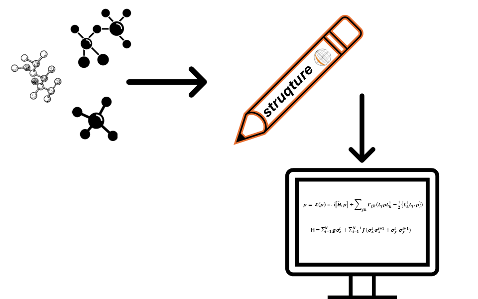
We describe decoherence by representing it with the Lindblad equation. The Lindblad equation is a master equation determining the time evolution of the density matrix. It is given by \[ \dot{\rho} = \mathcal{L}(\rho) =-i [\hat{H}, \rho] + \sum_{j,k} \Gamma_{j,k} \left( L_{j}\rho L_{k}^{\dagger} - \frac{1}{2} \{ L_k^{\dagger} L_j, \rho \} \right) \] with the rate matrix \(\Gamma_{j,k}\) and the Lindblad operator \(L_{j}\).
To describe spin noise we use the Lindblad equation with \(\hat{H}=0\).
Therefore, to describe the pure noise part of the Lindblad equation one needs the rate matrix in a well defined basis of Lindblad operators.
We use the modified Pauli matrices {X, iY, Z} (DecoherenceProducts) as the operator basis.
The rate matrix and Lindblad noise model are saved as a sum over pairs of spin terms, giving the operators acting from the left and right on the density matrix.
In programming terms, the object PauliLindbladNoiseOperator is given by a HashMap or Dictionary with the tuple (DecoherenceProduct, DecoherenceProduct) as keys and the entries in the rate matrix as values.
Example
Here, we add the terms \( L_0 = \sigma_0^{x} \sigma_1^{z} \) and \( L_1 = \sigma_0^{x} \sigma_2^{z} \) with coefficient 1.0:
\[ \hat{O}_{noise}(\rho) = 1.0 \left( L_0 \rho L_1^{\dagger} - \frac{1}{2} \{ L_1^{\dagger} L_0, \rho \} \right) \]
from struqture_py import spins

# We start by initializing the PauliLindbladNoiseOperator
noise_operator = spins.PauliLindbladNoiseOperator()

# Adding in the (0X1Z, 0X2Z) term
noise_operator.set(("0X1Z", "0X2Z"), 1.0)
print(noise_operator)

# As with the coherent operators, the `set` function overwrites any existing value for the given key (here, a tuple of strings or DecoherenceProducts).
# Should you prefer to use and additive method, please use `add_operator_product`:
noise_operator.add_operator_product(("0X1Z", "0X2Z"), 1.0)
# NOTE: this is equivalent to: noise_operator.add_operator_product((PauliProduct().x(0).z(1), PauliProduct().x(0).z(2)), 1.0)
Open systems
Open systems are quantum systems coupled to an environment that can often be described using Lindblad-type noise.
The Lindblad master equation is given by
\[
\dot{\rho} = \mathcal{L}(\rho) =-i [\hat{H}, \rho] + \sum_{j,k} \Gamma_{j,k} \left( L_{j}\rho L_{k}^{\dagger} - \frac{1}{2} \{ L_k^{\dagger} L_j, \rho \} \right)
\]
In struqture they are composed of a hamiltonian (PauliHamiltonian) and noise (PauliLindbladNoiseOperator), representing the first and second parts of the equation (respectively).
Example
from struqture_py import spins

# We start by initializing our PauliLindbladOpenSystem
open_system = spins.PauliLindbladOpenSystem()

# Set the sigma_1^z term into the system part of the open system
open_system.system_set("1Z", 2.0)
# Set the sigma_0^x sigma_2^z term into the noise part of the open system
open_system.noise_set(("0X2Z", "0X2Z"), 1.5)

# Please note that the `system_set` and `noise_set` functions will set the values given, overwriting any previous value.
# Should you prefer to use and additive method, please use `system_add_operator_product` and `noise_add_operator_product`:
open_system.system_add_operator_product("1Z", 2.0)
open_system.noise_add_operator_product(("0X2Z", "0X2Z"), 1.5)

print(open_system)
Applied Examples
Struqture can be used in a variety of contexts, some of which are detailed below.
NMR
HQS NMR
Struqture can be used in conjunction with the HQS NMR package, to calculate NMR correlators for Hamiltonians. This is shown in the following examples:
- Simulate a small-scale Hamiltonian from struqture (json) on a quantum computer
- Simulate an NMR spectrum from a struqture Hamiltonian
- Solving spin lattice models using struqture
Please note that the notebooks linked above are pre-run, as they require the HQS NMR python package. Should you wish to run them yourself, please install the HQS NMR package using the install instructions and download the accompanying HQS NMR examples.
Matrix Representation
All spin-objects can be converted into sparse matrices with the following convention. If \(M_2\) corresponds to the matrix acting on spin 2 and \(M_1\) corresponds to the matrix acting on spin 1 the total matrix \(M\) acting on spins 0 to 2 is given by \[ M = M_2 \otimes M_1 \otimes \mathbb{1} \] For an \(N\)-spin operator a term acts on the \(2^N\) dimensional space of state vectors. A superoperator operates on the \(4^N\) dimensional space of flattened density-matrices. struqture uses the convention that density matrices are flattened in row-major order \[ \rho = \begin{pmatrix} a & b \\ c & d \end{pmatrix} => \vec{\rho} = \begin{pmatrix} a \\ b \\ c \\ d \end{pmatrix} \]
Hamiltonians and Operators
For noiseless objects (PauliOperator, PauliHamiltonian), sparse operators and sparse superoperators can be constructed, as we can represent the operator as a wavefunction.
Note that the matrix representation functionality exists only for spin objects, and can’t be generated for bosonic, fermionic or mixed system objects.
from struqture_py import spins
from scipy.sparse import coo_matrix

# We start by building the operator we want to represent
operator = spins.PauliOperator()
operator.add_operator_product("0Z1Z", 0.5)

# Using the `sparse_matrix_coo` function, we can
# return the information in scipy coo_matrix form, which can be directly fed in:
python_coo = coo_matrix(operator.sparse_matrix_coo(number_spins=2))
print(python_coo.todense())
Open Systems and Noise Operators
For operators with noise (PauliLindbladNoiseOperator, PauliLindbladOpenSystem), however, we can only represent them as matrices operating on density matrices (in vector form) and can therefore only construct sparse superoperators.
Note that the matrix representation functionality exists only for spin objects, and can’t be generated for bosonic, fermionic or mixed system objects.
from struqture_py import spins
from scipy.sparse import coo_matrix

# We start by building the noise operator we want to represent
operator = spins.PauliLindbladNoiseOperator()
operator.add_operator_product(("0X2Z", "0X2Z"), 1.0 + 1.5j)

# Using the `sparse_matrix_coo` function, we can
# return the information in scipy coo_matrix form, which can be directly fed in:
python_coo = coo_matrix(operator.sparse_matrix_superoperator_coo(number_spins=3))
print(python_coo.todense())
Advanced Users
Welcome to the Advanced Users section of the user documentation for spins. We invite you to peruse the following topics:
- Alternative representation {+, -, z}
- Using symbolic parameters
- Building blocks: PauliProduct and DecoherenceProduct
For further advanced topics, please consult the Struqture design & implementation section.
The {+, -, z} basis
The basis itself
The {+, -, z} basis is defined as follows:
-
I: identity matrix \[ \begin{pmatrix} 1 & 0\\ 0 & 1 \end{pmatrix} \]
-
+: \( \sigma^+ = \frac{1}{2} ( \sigma^x + \mathrm{i} \sigma^y ) \) \[ \begin{pmatrix} 0 & 1\\ 0 & 0 \end{pmatrix} \]
-
-: \( \sigma^- = \frac{1}{2} ( \sigma^x - \mathrm{i} \sigma^y ) \) \[ \begin{pmatrix} 0 & 0\\ 1 & 0 \end{pmatrix} \]
-
Z: \( \sigma^z \) matrix \[ \begin{pmatrix} 1 & 0\\ 0 & -1 \end{pmatrix} \]
Symbolic representation and PlusMinusProduct
The following lines of code are equivalent ways to represent these matrices acting on spin indices, when passing them to the operators described in the rest of this section:
from struqture_py.spins import PlusMinusProduct

product = PlusMinusProduct().plus(0).minus(1).z(2)  # these can be chained similarly to PauliProducts
product = "0+1-2Z"
Note that when using setter methods as in PlusMinusProduct().z(0), the methods set the value of the operator acting on the corresponding spin and do not
represent matrix multiplication, so that PlusMinusProduct().z(0) is equivalent to PlusMinusProduct().z(0).z(0), the second call to the setter method z(0) having no effect.
Operators
PlusMinusOperators represent operators such as:
\[
\hat{O} = \sum_{j} \alpha_j \prod_{k=0}^N \sigma_{j, k} \\
\sigma_{j, k} \in \{ +_k, -_k, Z_k, I_k \} .
\]
From a programming perspective the operators are HashMaps or Dictionaries with the PlusMinusProducts as keys and the coefficients \(\alpha_j\) as values.
Example
Here is an example of how to build a PlusMinusOperator:
from struqture_py import spins

# We would like to build the following operator:
# O = (1 + 1.5 * i) * sigma^+_0 * sigma^z_2

# We start by initializing our PlusMinusOperator
operator = spins.PlusMinusOperator()
# We set the term and value specified above
operator.set("0+2Z", 1.0 + 1.5j)
# We can use the `get` function to check what value/prefactor is stored for 0+2Z
assert operator.get("0+2Z") == complex(1.0, 1.5)
print(operator)

# Please note that the `set` function will set the value given, overwriting any previous value.
# Should you prefer to use and additive method, please use `add_operator_product`:
operator.add_operator_product("0+2Z", 1.0)
# NOTE: this is equivalent to: operator.add_operator_product(PlusMinusProduct().plus(0).z(2), 1.0)
print(operator)

# NOTE: the above values used can also be symbolic.
# Symbolic parameters can be very useful for a variety of reasons, as detailed in the introduction.
operator.add_operator_product("0Z1Z", "parameter")
Mathematical operations
The available mathematical operations for PlusMinusOperator are demonstrated below:
from struqture_py.spins import PlusMinusOperator

# Setting up two test PlusMinusOperators
operator_1 = PlusMinusOperator()
operator_1.add_operator_product("0+", 1.5j)

operator_2 = PlusMinusOperator()
operator_2.add_operator_product("2Z3Z", 0.5)

# Addition & subtraction:
operator_3 = operator_1 - operator_2
operator_3 = operator_3 + operator_1

# Multiplication:
operator_1 = operator_1 * 2.0
operator_4 = operator_1 * operator_2
Matrix representation: spin objects only
All spin-objects can be converted into sparse matrices with the following convention.
If \(M_2\) corresponds to the matrix acting on spin 2 and \(M_1\) corresponds to the matrix acting on spin 1 the total matrix \(M\) acting on spins 0 to 2 is given by
\[
M = M_2 \otimes M_1 \otimes \mathbb{1}
\]
For an \(N\)-spin operator a term acts on the \(2^N\) dimensional space of state vectors.
A superoperator operates on the \(4^N\) dimensional space of flattened density-matrices.
struqture uses the convention that density matrices are flattened in row-major order
\[
\rho = \begin{pmatrix} a & b \\ c & d \end{pmatrix} => \vec{\rho} = \begin{pmatrix} a \\ b \\ c \\ d \end{pmatrix}
\]
For noiseless objects (PlusMinusOperator), sparse operators and sparse superoperators can be constructed, as we can represent the operator as a wavefunction.
Note that the matrix representation functionality exists only for spin objects, and can’t be generated for bosonic, fermionic or mixed system objects.
from struqture_py import spins
from scipy.sparse import coo_matrix

# We start by building the operator we want to represent
operator = spins.PlusMinusOperator()
operator.add_operator_product("0Z1Z", 0.5)

# Using the `sparse_matrix_coo` function, we can
# return the information in scipy coo_matrix form, which can be directly fed in:
python_coo = coo_matrix(operator.sparse_matrix_coo(number_spins=2))
print(python_coo.todense())
Noise Operators
We describe decoherence by representing it with the Lindblad equation. The Lindblad equation is a master equation determining the time evolution of the density matrix. It is given by \[ \dot{\rho} = \mathcal{L}(\rho) =-i [\hat{H}, \rho] + \sum_{j,k} \Gamma_{j,k} \left( L_{j}\rho L_{k}^{\dagger} - \frac{1}{2} \{ L_k^{\dagger} L_j, \rho \} \right) \] with the rate matrix \(\Gamma_{j,k}\) and the Lindblad operator \(L_{j}\).
To describe spin noise we use the Lindblad equation with \(\hat{H}=0\).
Therefore, to describe the pure noise part of the Lindblad equation one needs the rate matrix in a well defined basis of Lindblad operators.
We use the {+, -, Z} matrices (PlusMinusProducts) as the operator basis.
The rate matrix and Lindblad noise model are saved as a sum over pairs of spin terms, giving the operators acting from the left and right on the density matrix.
In programming terms, the object PlusMinusLindbladNoiseOperator is given by a HashMap or Dictionary with the tuple (PlusMinusProduct, PlusMinusProduct) as keys and the entries in the rate matrix as values.
Example
Here, we add the terms \( L_0 = \sigma_0^{+} \sigma_1^{z} \) and \( L_1 = \sigma_0^{+} \sigma_2^{z} \) with coefficient 1.0: \[ \hat{O}_{noise}(\rho) = 1.0 \left( L_0 \rho L_1^{\dagger} - \frac{1}{2} \{ L_1^{\dagger} L_0, \rho \} \right) \]
from struqture_py import spins

# We start by initializing the PlusMinusLindbladNoiseOperator
operator = spins.PlusMinusLindbladNoiseOperator()

# Adding in the (0+1Z, 0+2Z) term
operator.set(("0+2Z", "0+2Z"), 1.0+1.5*1j)
print(operator)

# As with the coherent operators, the `set` function overwrites any existing value for the given key (here, a tuple of strings or PlusMinusProducts).
# Should you prefer to use and additive method, please use `add_operator_product`:
operator.add_operator_product(("0+1Z", "0+2Z"), 1.0)
# NOTE: this is equivalent to: operator.add_operator_product((PlusMinusProduct().plus(0).z(1), PlusMinusProduct().plus(0).z(2)), 1.0)
Symbolic parameters
Symbolic parameters, or parametrisation of the classes, can be very useful for users creating Hamiltonians or operators with different coupling/on-site/… strengths.
Example
For instance, if a user would like to define the following Hamiltonian:
\[ \hat{H} = J \sum_{i, j} \sigma_x^i \sigma_x^j + \alpha \sum_i \sigma_z^i \]
where the values for \(J\) range between [-1.0, 1.0] and the values for \( \alpha \) range between [0.2, 0.4], the user might try to define all these Hamiltonians one at a time. However, with struqture, the user can define the Hamiltonian once, passing symbolic parameters "J" and "alpha" as the coefficients, and substituting them for the correct values in situ, later. We show an example of this below, where we pass our symbolic Hamiltonian to our closed-source software, the HQS Quantum Libraries. These then create the circuit representing the Trotterised time evolution corresponding to the Hamiltonian, and then substitute the "J" and "alpha" values at each Trotter time step. We can then go on to simulate this circuit, now that the symbolic parameters have been substituted.
from struqture_py.spins import PauliHamiltonian
from hqs_quantum_libraries import alqorithms

# Defining the base Hamiltonian
hamiltonian = PauliHamiltonian()
number_spins = 4
for i in range(number_spins):
    for j in (i + 1, number_spins):
        hamiltonian.add_operator_product(f"{i}X{j}X", "J")
for i in range(number_spins):
    hamiltonian.add_operator_product(f"{i}Z", "alpha")

print(hamiltonian)

# This Hamiltonian can then be used later in the following fashion:
algorithm = py_alqorithms.QSWAPAlgorithm(1)
time = 1.0
for (j_coupling, alpha_coupling) in zip(range(-1.0, 1.0), range(0.2, 0.4)):
    # turn the hamiltonian into a quantum Circuit (see the qoqo documentation) using the HQS Quantum Libraries
    circuit = algorithm.create_circuit(hamiltonian, time)
    circuit_to_run = circuit.substitute_parameters({"J": j_coupling, "alpha": alpha_coupling})
    # run circuit on hardware or on a simulator
Complex Symbolic Parameters
A note on complex parameters: we have several classes (PauliOperator, PauliLindbladNoiseOperator) that take complex parameters when building them.
These can also be made symbolic:
- if the entire parameter (real + imaginary parts) is symbolic, the same code as above can be used: a string is passed instead of a number when adding a product to the operator.
- if only a part (real part or imaginary part) is symbolic, while the other part is a number, the user must use the CalculatorComplex class (
qoqo_calculator_pyo3package). This is demonstrated below.
from struqture_py.spins import PauliOperator
from qoqo_calculator_pyo3 import CalculatorComplex

operator = PauliOperator()
operator.add_operator_product("0Z1Z", CalculatorComplex.from_pair("a", 1.0))  # This sets: a + i * 1.0
operator.add_operator_product("0X", CalculatorComplex.from_pair(1.0, "a"))  # This set 1.0 + i * a
operator.add_operator_product("1X", CalculatorComplex.from_pair("b", "c")) # This sets b + i * c. Please note that b and c will need to be substituted separately.
Advanced Users: PauliProducts and DecoherenceProducts
Up until this point, we have shown how to pass terms to a Hamiltonian or operator using symbolic (string) representation. However, the underlying class is the PauliProduct and DecoherenceProduct (for coherent and incoherent dynamics, respectively).
NOTE: all of our higher-level objects accept both PauliProducts/DecoherenceProducts (depending on the object) as well as symbolic notation. If the user is just getting started using struqture, we recommend using the symbolic notation and skipping this section of the documentation, starting instead with the coherent dynamics section.
PauliProducts and DecoherenceProducts are the components that users utilise to create spin terms, e.g. \( \sigma_0^x \sigma_1^x \).
PauliProducts can later be combined to create operators or Hamiltonians (see the coherent dynamics section), while DecoherenceProducts can be combined to create noise operators or open systems (see the incoherent dynamics section).
Definitions
The products are built by setting the operators acting on separate spins.
PauliProducts are combinations of SinglePauliOperators on specific spin indices. These are the SinglePauliOperators, or Pauli matrices, as defined in the introductory section. The same applies to the DecoherenceProducts and their SingleDecoherenceOperators.
Example
In Python the separate operators can be set via functions. In the python interface a PauliProduct can often be replaced by its unique string representation.
Note that when using setter methods as in PauliProduct().x(0), the methods set the value of the Pauli operator acting on the corresponding spin and do not
represent matrix multiplication, so that PauliProduct().x(0) is equivalent to PauliProduct().x(0).x(0), the second call to the setter method x(0) having no effect.
from struqture_py.spins import PauliProduct, DecoherenceProduct

# We can build single-spin terms:
sigma_x_0 = PauliProduct().x(0)  # sigma_x acting on spin 0
sigma_y_1 = PauliProduct().y(1)  # sigma_y acting on spin 1
sigma_z_2 = PauliProduct().z(2)  # sigma_z acting on spin 2

# As well as two-spin terms:
sigma_x_0_x_1 = PauliProduct().x(0).x(1)  # sigma_x acting on spin 0 and spin 1
sigma_y_1_z_20 = PauliProduct().y(1).z(20)  # sigma_y acting on spin 1 and sigma_z spin 20
# We can also initialize the PauliProducts from string:
sigma_y_1_z_20 = PauliProduct.from_string("1Y20Z")

# We can chain as many of these as we would like!
# A product of a X acting on spin 0, a Y acting on spin 3 and a Z acting on spin 20
pp = PauliProduct().x(0).y(3).z(20)
# This is equivalent to the string representation
pp_string = str(pp)

# The same functionality is available for DecoherenceProducts.
# **NOTE**: The name of the y() becomes .iy() for DecoherenceProducts to match the change in matrix representation
# A product of a X acting on spin 0, a iY acting on spin 3 and a Z acting on spin 20
dp = DecoherenceProduct().x(0).iy(3).z(20)
# Often equivalent to the string representation
dp_string = str(dp)
Non-spin objects
Struqture also supports non-spin systems. The following object families are currently available:
- bosonic modes
- fermionic modes
- mixed systems: these classes allow combinations of spins, bosonic modes, and fermionic modes within a single model.
As with spin objects, these types can be instantiated programmatically or loaded from a file, and once constructed they can be used in the same manner as user-created objects. Refer to the respective sections for details on available constructors, operators, getters, setters, and properties.
Bosons
Struqture can be used to represent bosonic operators and hamiltonians, such as:
\[ \hat{O} = \sum_{j=0}^N \alpha_j \left( \prod_{k=0}^N f(j, k) \right) \left( \prod_{l=0}^N g(j, l) \right) \] with \[ f(j, k) = \begin{cases} b_k^{\dagger} \\ \mathbb{1} \end{cases} , \] \[ g(j, l) = \begin{cases} b_l \\ \mathbb{1} \end{cases} , \] or an open system given by its Lindblad desription \[ \dot{\rho} = \mathcal{L}(\rho) = -i [\hat{H}, \rho] + \sum_{j,k} \Gamma_{j,k} \left( L_{j}\rho L_{k}^{\dagger} - \frac{1}{2} \{ L_k^{\dagger} L_j, \rho \} \right) \]
The simplest way that the user can interact with these matrices is by using symbolic representation: "c0a0" represents a \( b^{\dagger}_0\ b_0 \) term. We use “c” to denote indices operated on by the creator operator and “a” to denote indices operated on by the annihilation operator. This is a very scalable approach, as indices not mentioned in this string representation are assumed to be acted on by the identity operator: "c7a25" represents a \( b^{\dagger}_7 b_{25} \) term, where all other terms (0 to 6 and 8 to 24) are acted on by \(I\).
However, for more fine-grain control over the operators, we invite the user to look into the BosonProduct and HermitianBosonProduct classes, in the Building blocks section. Otherwise please proceed to the coherent or decoherent dynamics section.
Bosons
Struqture can be used to represent bosonic operators and hamiltonians, such as:
\[ \hat{O} = \sum_{j=0}^N \alpha_j \left( \prod_{k=0}^N f(j, k) \right) \left( \prod_{l=0}^N g(j, l) \right) \] with \[ f(j, k) = \begin{cases} b_k^{\dagger} \\ \mathbb{1} \end{cases} , \] \[ g(j, l) = \begin{cases} b_l \\ \mathbb{1} \end{cases} , \] or an open system given by its Lindblad desription \[ \dot{\rho} = \mathcal{L}(\rho) = -i [\hat{H}, \rho] + \sum_{j,k} \Gamma_{j,k} \left( L_{j}\rho L_{k}^{\dagger} - \frac{1}{2} \{ L_k^{\dagger} L_j, \rho \} \right) \]
The simplest way that the user can interact with these objects is by using symbolic representation: "c0a0" represents a \( b^{\dagger}_0\ b_0 \) term. We use “c” to denote indices operated on by the creator operator and “a” to denote indices operated on by the annihilation operator. This is a very scalable approach, as indices not mentioned in this string representation are assumed to be acted on by the identity operator: "c7a25" represents a \( b^{\dagger}_7 b_{25} \) term, where all other terms (0 to 6 and 8 to 24) are acted on by \(I\).
However, for more fine-grain control over the operators, we invite the user to look into the BosonProduct and HermitianBosonProduct classes, in the Building blocks section. Otherwise, please proceed to the coherent or decoherent dynamics section.
Operators and Hamiltonians
BosonOperators and BosonHamiltonians represent operators or Hamiltonians such as:
\[ \hat{O} = \sum_{j=0}^N \alpha_j \left( \prod_{k=0}^N f(j, k) \right) \left( \prod_{l=0}^N g(j, l) \right) \]
with
\[ f(j, k) = \begin{cases} b_k^{\dagger} \\ \mathbb{1} \end{cases} , \]
\[ g(j, l) = \begin{cases} b_l \\ \mathbb{1} \end{cases} , \]
and
\(b^{\dagger}\) the bosonic creation operator, \(c\) the bosonic annihilation operator
\[ \lbrack b_k^{\dagger}, b_j^{\dagger} \rbrack = 0, \\
\lbrack b_k, b_j \rbrack = 0, \\
\lbrack b_k^{\dagger}, b_j \rbrack = \delta_{k, j}. \]
From a programming perspective the operators and Hamiltonians are HashMaps or Dictionaries with BosonProducts or HermitianBosonProducts (respectively) as keys and the coefficients \(\alpha_j\) as values.
In struqture we distinguish between bosonic operators and Hamiltonians to avoid introducing unphysical behaviour by accident.
While both are sums over normal ordered bosonic products (stored as dictionaries of products with a complex prefactor), Hamiltonians are guaranteed to be hermitian. In a bosonic Hamiltonian, this means that the sums of products are sums of hermitian bosonic products (we have not only the \(b^{\dagger}b\) terms but also their hermitian conjugate) and the on-diagonal terms are required to have real prefactors.
In the HermitianBosonProducts, we only explicitly store one part of the hermitian bosonic product, and we have chosen to store the one which has the smallest index of the creators that is smaller than the smallest index of the annihilators. For instance, if the user would like to define a \(b_0^{\dagger} + b_0\) term, they would create this object: HermitianBosonProduct([], [0]). The second part of the term is stored implicitly by the code.
Example
Here is an example of how to build a BosonOperator:
from struqture_py import bosons

# We start by initializing our BosonOperator
operator = bosons.BosonOperator()

# We set the term and some value of our choosing
operator.set("c0c1a0a2", 1.0 + 1.5j)
# We can use the `get` function to check what value/prefactor is stored for the BosonProduct
assert operator.get("c0c1a0a2") == complex(1.0, 1.5)
print(operator)

# Please note that the `set` function will set the value given, overwriting any previous value.
# Should you prefer to use and additive method, please use `add_operator_product`:
operator.add_operator_product("c0c1a0a2", 1.0)
print(operator)
# NOTE: this is equivalent to: operator.add_operator_product(BosonProduct([0, 1], [0, 2]))

# NOTE: the above values used can also be symbolic.
# Symbolic parameters can be very useful for a variety of reasons, as detailed in the introduction.
operator.add_operator_product(hbp, "parameter")
Here is an example of how to build a BosonHamiltonian:
from struqture_py import bosons

# We start by initializing our BosonHamiltonian
hamiltonian = bosons.BosonHamiltonian()
# We set both of the terms and values specified above
hamiltonian.set("c0a0", 0.5)
hamiltonian.set("c1a1", 0.5)

# Please note that the `set` function will set the value given, overwriting any previous value.
# Should you prefer to use and additive method, please use `add_operator_product`:
hamiltonian.add_operator_product("c0a0", 1.0)

print(hamiltonian)

# NOTE: the above values used can also be symbolic.
# Symbolic parameters can be very useful for a variety of reasons, as detailed in the introduction.
hamiltonian.add_operator_product("c0a0", "parameter")
Noise operators
We describe decoherence by representing it with the Lindblad equation. The Lindblad equation is a master equation determining the time evolution of the density matrix. It is given by \[ \dot{\rho} = \mathcal{L}(\rho) = -i [\hat{H}, \rho] + \sum_{j,k} \Gamma_{j,k} \left( L_{j}\rho L_{k}^{\dagger} - \frac{1}{2} \{ L_k^{\dagger} L_j, \rho \} \right) \] with the rate matrix \(\Gamma_{j,k}\) and the Lindblad operator \(L_{j}\).
To describe bosonic noise we use the Lindblad equation with \(\hat{H}=0\).
Therefore, to describe the pure noise part of the Lindblad equation one needs the rate matrix in a well defined basis of Lindblad operators.
We use BosonProducts as the operator basis.
The rate matrix and with it the Lindblad noise model is saved as a sum over pairs of BosonProducts, giving the operators acting from the left and right on the density matrix.
In programming terms the object BosonLindbladNoiseOperator is given by a HashMap or Dictionary with the tuple (BosonProduct, BosonProduct) as keys and the entries in the rate matrix as values.
Example
Here, we add the terms \(L_0 = b^{\dagger}_0 b_0\) and \(L_1 = b^{\dagger}_0 b_1\) with coefficient 1.0: \( 1.0 \left( L_0 \rho L_1^{\dagger} - \frac{1}{2} \{ L_1^{\dagger} L_0, \rho \} \right) \)
from struqture_py import bosons

# We start by initializing the BosonLindbladNoiseOperator
operator = bosons.BosonLindbladNoiseOperator()

# Adding in the (b^{\dagger}_0 * b_0, b^{\dagger}_0 * b_1) term
operator.set(("c0a0", "c0a1"), 1.0 + 1.5 * 1j)
print(operator)

# As with the coherent operators, the `set` function overwrites any existing value for the given key (here, a tuple of strings or DecoherenceProducts).
# Should you prefer to use and additive method, please use `add_operator_product`:
operator.add_operator_product(("c0a0", "c0a1"), 1.0)
# NOTE: this is equivalent to: operator.add_operator_product((bosonProduct([0], [0]), bosonProduct([0], [1])), 1.0)
Open systems
Physically open systems are quantum systems coupled to an environment that can often be described using Lindblad type of noise.
The Lindblad master equation is given by
\[
\dot{\rho} = \mathcal{L}(\rho) =-i [\hat{H}, \rho] + \sum_{j,k} \Gamma_{j,k} \left( L_{j}\rho L_{k}^{\dagger} - \frac{1}{2} \{ L_k^{\dagger} L_j, \rho \} \right)
\]
In struqture they are composed of a Hamiltonian (BosonHamiltonian) and noise (BosonLindbladNoiseOperator). They have different ways to set terms in Rust and Python:
Example
from struqture_py import bosons

# We start by initializing our BosonLindbladOpenSystem
open_system = bosons.BosonLindbladOpenSystem()

# Set the c_b^{\dagger}_0 * c_b_0 term into the system part of the open system
open_system.system_set("c0a0", 2.0)
# Set the b^{\dagger}_0 * b^{\dagger}_1 * b_0 * b_1 b^{\dagger}_0 * b^{\dagger}_1 * b_0 * b_2 term into the noise part of the open system
open_system.noise_set(("c0c1a0a1", "c0c1a0a2"), 1.5)

# Please note that the `system_set` and `noise_set` functions will set the values given, overwriting any previous value.
# Should you prefer to use and additive method, please use `system_add_operator_product` and `noise_add_operator_product`:
open_system.system_add_operator_product("c0a0", 2.0)
open_system.noise_add_operator_product(("c0c1a0a1", "c0c1a0a2"), 1.5)

print(open_system)
Overview
All bosonic objects in struqture are expressed based on products of bosonic creation and annihilation operators, which respect bosonic commutation relations
\[ \lbrack b_k^{\dagger}, b_j^{\dagger} \rbrack = 0, \\
\lbrack b_k, b_j \rbrack = 0, \\
\lbrack b_k, b_j^{\dagger} \rbrack = \delta_{k, j}. \]
NOTE: all of our higher-level objects accept BosonProducts/HermitianBosonProducts (depending on the object) as well as symbolic notation. If the user is just getting started using struqture, we recommend using the symbolic notation and skipping this section of the documentation for now, starting instead with the coherent dynamics section.
BosonProducts
BosonProducts are simple combinations of bosonic creation and annihilation operators.
HermitianBosonProducts
HermitianBosonProducts are the hermitian equivalent of BosonProducts. This means that even though they are constructed the same (see the next section, Examples), they internally store both that term and its hermitian conjugate. For instance, given the term \(b^{\dagger}_0 b_1 b_2\), a BosonProduct would represent \(b^{\dagger}_0 b_1 b_2\) while a HermitianBosonProduct would represent \(c^{\dagger}_0 b_1 b_2 + b^{\dagger}_2 b^{\dagger}_1 b_0\).
Example
The operator product is constructed by passing an array or a list of integers to represent the creation indices, and an array or a list of integers to represent the annihilation indices.
Note: (Hermitian)BosonProducts can only been created from the correct ordering of indices (the wrong sequence will return an error) but we have the create_valid_pair function to create a valid Product from arbitrary sequences of operators which also transforms an index value according to the commutation and hermitian conjugation rules.
from struqture_py.bosons import BosonProduct, HermitianBosonProduct

# A product of a creation operator acting on bosonic mode 0 and an annihilation operator
# acting on bosonic mode 20
bp = BosonProduct([0], [20])
# Building the term b^{\dagger}_1 * b^{\dagger}_3 * b_0
bp = BosonProduct.create_valid_pair([3, 1], [0], 1.0)


# A product of a creation operator acting on bosonic mode 0 and an annihilation
# operator acting on bosonic mode 20, as well as a creation operator acting on
# bosonic mode 20 and an annihilation operator acting on bosonic mode 0
hbp = HermitianBosonProduct([0], [20])
# Building the term b^{\dagger}_0 * b^{\dagger}_3 * b_0 + b^{\dagger}_0 * b_3 * b_0
hbp = HermitianBosonProduct.create_valid_pair([3, 0], [0], 1.0)
Fermions
Struqture can be used to represent Fermion operators, hamiltonians and open systems, such as:
\[ \hat{O} = \sum_{j=0}^N \alpha_j \left( \prod_{k=0}^N f(j, k) \right) \left( \prod_{l=0}^N g(j, l) \right) \] with \[ f(j, k) = \begin{cases} c_k^{\dagger} \\ \mathbb{1} \end{cases} , \] \[ g(j, l) = \begin{cases} c_l \\ \mathbb{1} \end{cases} , \] and \[ \dot{\rho} = \mathcal{L}(\rho) = -i [\hat{H}, \rho] + \sum_{j,k} \Gamma_{j,k} \left( L_{j}\rho L_{k}^{\dagger} - \frac{1}{2} \{ L_k^{\dagger} L_j, \rho \} \right) \]
The simplest way that the user can interact with these matrices is by using symbolic representation: "c0a0" represents a \( c^{\dagger}_0\ c_0 \) term.
Note: Here c is used in the equations to represent any fermion operator while b was used to represent a boson operator. However, in string serialisation strquture uses the convention that c always represents a creation operator, whether in the fermionic or bosonic degrees of freedom and a always represents an annihilation operator.
This is a very scalable approach, as indices not mentioned in this string representation are assumed to be acted on by the identity operator: "c7a25" represents a \( c^{\dagger}_7 c_{25} \) term, where all other terms (0 to 6 and 8 to 24) are acted on by \(I\).
However, for more fine-grain control over the operators, we invite the user to look into the FermionProduct and HermitianFermionProduct classes, in the Building blocks section. Otherwise please proceed to the coherent or decoherent dynamics section.
Fermions
Struqture can be used to represent Fermion operators, hamiltonians and open systems, such as:
\[ \hat{O} = \sum_{j=0}^N \alpha_j \left( \prod_{k=0}^N f(j, k) \right) \left( \prod_{l=0}^N g(j, l) \right) \] with \[ f(j, k) = \begin{cases} c_k^{\dagger} \\ \mathbb{1} \end{cases} , \] \[ g(j, l) = \begin{cases} c_l \\ \mathbb{1} \end{cases} , \] and \[ \dot{\rho} = \mathcal{L}(\rho) = -i [\hat{H}, \rho] + \sum_{j,k} \Gamma_{j,k} \left( L_{j}\rho L_{k}^{\dagger} - \frac{1}{2} \{ L_k^{\dagger} L_j, \rho \} \right) \]
The simplest way that the user can interact with these objects is by using symbolic representation: "c0a0" represents a \( c^{\dagger}_0\ c_0 \) term.
Note: Here c is used in the equations to represent any fermion operator while b was used to represent a boson operator. However, in string serialisation strquture uses the convention that c always represents a creation operator, whether in the fermionic or bosonic degrees of freedom and a always represents an annihilation operator.
This is a very scalable approach, as indices not mentioned in this string representation are assumed to be acted on by the identity operator: "c7a25" represents a \( c^{\dagger}_7 c_{25} \) term, where all other terms (0 to 6 and 8 to 24) are acted on by \(I\).
However, for more fine-grain control over the operators, we invite the user to look into the FermionProduct and HermitianFermionProduct classes, in the Building blocks section. Otherwise please proceed to the coherent or decoherent dynamics section.
Operators and Hamiltonians
FermionOperators and FermionHamiltonians represent operators or Hamiltonians such as:
\[ \hat{O} = \sum_{j=0}^N \alpha_j \left( \prod_{k=0}^N f(j, k) \right) \left( \prod_{l=0}^N g(j, l) \right) \]
with
\[ f(j, k) = \begin{cases} c_k^{\dagger} \\ \mathbb{1} \end{cases} , \]
\[ g(j, l) = \begin{cases} c_l \\ \mathbb{1} \end{cases} , \]
and
\(c^{\dagger}\) the fermionionic creation operator, \(c\) the fermionionic annihilation operator
\[ \lbrace c_k^{\dagger}, c_j^{\dagger} \rbrace = 0, \\
\lbrace c_k, c_j \rbrace = 0, \\
\lbrace c_k^{\dagger}, c_j \rbrace = \delta_{k, j}. \]
For instance, \(c^{\dagger}_0 c^{\dagger}_1 c_1\) is a term with a \(c^{\dagger}\) term acting on 0, and both a \(c^{\dagger}\) term and a \(c\) term acting on 1.
From a programming perspective the operators and Hamiltonians are HashMaps or Dictionaries with FermionProducts or HermitianFermionProducts (respectively) as keys and the coefficients \(\alpha_j\) as values.
In struqture we distinguish between fermionic operators and Hamiltonians to avoid introducing unphysical behaviour by accident.
While both are sums over normal ordered fermionic products (stored as dictionaries of products with a complex prefactor), Hamiltonians are guaranteed to be hermitian. In a fermionic Hamiltonian, this means that the sums of products are sums of hermitian fermionic products (we have not only the \(c^{\dagger}c\) terms but also their hermitian conjugate) and the on-diagonal terms are required to have real prefactors.
In the HermitianFermionProducts, we only explicitly store one part of the hermitian fermionic product, and we have chosen to store the one which has the smallest index of the creators that is smaller than the smallest index of the annihilators. For instance, if the user would like to define a \(c_0^{\dagger} + c_0\) term, they would create this object: HermitianFermionProduct([], [0]). The second part of the term is stored implicitly by the code.
Example
Here is an example of how to build a FermionOperator:
from struqture_py import fermions

# We start by initializing our FermionOperator
operator = fermions.FermionOperator()

# We set the term and some value of our choosing
operator.set("c0c1a0a2", 1.0 + 1.5j)
# We can use the `get` function to check what value/prefactor is stored for the FermionProduct
assert operator.get("c0c1a0a2") == complex(1.0, 1.5)
print(operator)

# Please note that the `set` function will set the value given, overwriting any previous value.
# Should you prefer to use and additive method, please use `add_operator_product`:
operator.add_operator_product("c0c1a0a2", 1.0)
print(operator)
# NOTE: this is equivalent to: operator.add_operator_product(FermionProduct([0, 1], [0, 2]))

# NOTE: the above values used can also be symbolic.
# Symbolic parameters can be very useful for a variety of reasons, as detailed in the introduction.
operator.add_operator_product("c0c1a0a2", "parameter")
Here is an example of how to build a FermionHamiltonian:
from struqture_py import fermions

# We start by initializing our FermionHamiltonian
hamiltonian = fermions.FermionHamiltonian()
# We set both of the terms and values specified above
hamiltonian.set("c0a0", 0.5)
hamiltonian.set("c1a1", 0.5)

# Please note that the `set` function will set the value given, overwriting any previous value.
# Should you prefer to use and additive method, please use `add_operator_product`:
hamiltonian.add_operator_product("c0a0", 1.0)

print(hamiltonian)

# NOTE: the above values used can also be symbolic.
# Symbolic parameters can be very useful for a variety of reasons, as detailed in the introduction.
hamiltonian.add_operator_product("c0a0", "parameter")
Noise operators
We describe decoherence by representing it with the Lindblad equation. The Lindblad equation is a master equation determining the time evolution of the density matrix. It is given by \[ \dot{\rho} = \mathcal{L}(\rho) = -i [\hat{H}, \rho] + \sum_{j,k} \Gamma_{j,k} \left( L_{j}\rho L_{k}^{\dagger} - \frac{1}{2} \{ L_k^{\dagger} L_j, \rho \} \right) \] with the rate matrix \(\Gamma_{j,k}\) and the Lindblad operator \(L_{j}\).
To describe fermionic noise we use the Lindblad equation with \(\hat{H}=0\).
Therefore, to describe the pure noise part of the Lindblad equation one needs the rate matrix in a well defined basis of Lindblad operators.
We use FermionProducts as the operator basis.
The rate matrix and with it the Lindblad noise model is saved as a sum over pairs of FermionProducts, giving the operators acting from the left and right on the density matrix.
In programming terms the object FermionLindbladNoiseOperator is given by a HashMap or Dictionary with the tuple (FermionProduct, FermionProduct) as keys and the entries in the rate matrix as values.
Example
Here, we add the terms \(L_0 = c^{\dagger}_0 c_0\) and \(L_1 = c^{\dagger}_0 c_0\) with coefficient 1.0: \( 1.0 \left( L_0 \rho L_1^{\dagger} - \frac{1}{2} \{ L_1^{\dagger} L_0, \rho \} \right) \)
from struqture_py import fermions

# We start by initializing the FermionLindbladNoiseOperator
operator = fermions.FermionLindbladNoiseOperator()

# Adding in the (c^{\dagger}_0 * c_0, c^{\dagger}_0 * c_1) term
operator.set(("c0a0", "c0a1"), 1.0 + 1.5 * 1j)
print(operator)

# As with the coherent operators, the `set` function overwrites any existing value for the given key (here, a tuple of strings or DecoherenceProducts).
# Should you prefer to use and additive method, please use `add_operator_product`:
operator.add_operator_product(("c0a0", "c0a1"), 1.0)
# NOTE: this is equivalent to: operator.add_operator_product((FermionProduct([0], [0]), FermionProduct([0], [1])), 1.0)
Open systems
Physically open systems are quantum systems coupled to an environment that can often be described using Lindblad type of noise.
The Lindblad master equation is given by
\[
\dot{\rho} = \mathcal{L}(\rho) =-i [\hat{H}, \rho] + \sum_{j,k} \Gamma_{j,k} \left( L_{j}\rho L_{k}^{\dagger} - \frac{1}{2} \{ L_k^{\dagger} L_j, \rho \} \right)
\]
In struqture they are composed of a Hamiltonian (FermionHamiltonian) and noise (FermionLindbladNoiseOperator).
Example
from struqture_py import fermions

# We start by initializing our FermionLindbladOpenSystem
open_system = fermions.FermionLindbladOpenSystem()

# Set the c^{\dagger}_0 * c_0 term into the system part of the open system
open_system.system_set("c0a0", 2.0)
# Set the c^{\dagger}_0 * c^{\dagger}_1 * c_0 * c_1 c^{\dagger}_0 * c^{\dagger}_1 * c_0 * c_2 term into the noise part of the open system
open_system.noise_set(("c0c1a0a1", "c0c1a0a2"), 1.5)

# Please note that the `system_set` and `noise_set` functions will set the values given, overwriting any previous value.
# Should you prefer to use and additive method, please use `system_add_operator_product` and `noise_add_operator_product`:
open_system.system_add_operator_product("c0a0", 2.0)
open_system.noise_add_operator_product(("c0c1a0a1", "c0c1a0a2"), 1.5)

print(open_system)
Overview
All fermionic objects in struqture are expressed based on products of fermionic creation and annihilation operators, which respect fermionic anti-commutation relations
\[ \lbrace c_k^{\dagger}, c_j^{\dagger} \rbrace = 0, \\
\lbrace c_k, c_j \rbrace = 0, \\
\lbrace c_k, c_j^{\dagger} \rbrace = \delta_{k, j}. \]
NOTE: all of our higher-level objects accept FermionProducts/HermitianFermionProducts (depending on the object) as well as symbolic notation. If the user is just getting started using struqture, we recommend using the symbolic notation and skipping this section of the documentation for now, starting instead with the coherent dynamics section.
FermionProducts
FermionProducts are simple combinations of fermionic creation and annihilation operators.
HermitianFermionProducts
HermitianFermionProducts are the hermitian equivalent of FermionProducts. This means that even though they are constructed the same (see the next section, Examples), they internally store both that term and its hermitian conjugate. For instance, given the term \(c^{\dagger}_0 c_1 c_2\), a FermionProduct would represent \(c^{\dagger}_0 c_1 c_2\) while a HermitianFermionProduct would represent \(c^{\dagger}_0 c_1 c_2 + c^{\dagger}_2 c^{\dagger}_1 c_0\).
Example
The operator product is constructed by passing an array or a list of integers to represent the creation indices, and an array or a list of integers to represent the annihilation indices.
Note: (Hermitian)FermionProducts can only been created from the correct ordering of indices (the wrong sequence will return an error) but we have the create_valid_pair function to create a valid Product from arbitrary sequences of operators which also transforms an index value according to the anti-commutation and hermitian conjugation rules.
from struqture_py.fermions import FermionProduct, HermitianFermionProduct

# A product of a creation operator acting on fermionic mode 0 and an
# annihilation operator acting on fermionic mode 20
fp = FermionProduct([0], [20])
# Building the term c^{\dagger}_1 * c^{\dagger}_3 * c_0
fp = FermionProduct.create_valid_pair([3, 1], [0], 1.0)


# A product of a creation operator acting on fermionic mode 0 and an annihilation
# operator acting on fermionic mode 20, as well as a creation operator acting on
# fermionic mode 20 and an annihilation operator acting on fermionic mode 0
hfp = HermitianFermionProduct([0], [20])
# Building the term c^{\dagger}_0 * c^{\dagger}_3 * c_0 + c^{\dagger}_0 * c_3 * c_0
hfp = HermitianFermionProduct.create_valid_pair([3, 0], [0], 1.0)
Mixed Systems
Struqture can be used to represent mixed operators, hamiltonians and open systems, such as: \[ \hat{H} = \sum_j \alpha_j \prod_k \sigma_{j, k} \prod_{l, m} b_{l, j}^{\dagger} b_{m, j} \prod_{r, s} c_{r, j}^{\dagger} c_{s, j} \] with commutation relations and cyclicity respected.
The simplest way that the user can interact with these matrices is by using symbolic representation: "S0Z:Bc0a1:Fc0a0" represents a \( \sigma^z\ b^{\dagger}_0 b_1\ c^{\dagger}_0\ c_0 \) term. In this string representation, each subsystem is defined by its type, and ends with a colon, in order to show where the next subsystem starts. The type is one of three options: “S” if it is a spin subsystem, “B” if it is a bosonic subsystem, and “F” if it is a fermionic subsystem.
This is a very scalable approach, as indices not mentioned in this string representation are assumed to be acted on by the identity operator: "S7Z:Bc7a25:Fc25a7" represents a \( \sigma^{z}_7\ b^{\dagger}_7 b_{25}\ c^{\dagger}_{25}\ c_7 \) term, where all other terms (0 to 6 and 8 to 24) are acted on by \(I\).
However, for more fine-grain control over the operators, we invite the user to look into the MixedProduct, HermitianMixedProducts and MixedDecoherenceProducts classes, in the Building blocks section. Otherwise please proceed to the coherent or decoherent dynamics section.
Operators and Hamiltonians
MixedOperators and MixedHamiltonians represent operators or Hamiltonians such as:
\[ \hat{H} = \sum_j \alpha_j \prod_k \sigma_{j, k} \prod_{l, m} b_{l, j}^{\dagger} b_{m, j} \prod_{r, s} c_{r, j}^{\dagger} c_{s, j} \]
with commutation relations and cyclicity respected.
From a programming perspective the operators and Hamiltonians are HashMaps or Dictionaries with MixedProducts or HermitianMixedProducts (respectively) as keys and the coefficients \(\alpha_j\) as values.
In struqture we distinguish between mixed operators and Hamiltonians to avoid introducing unphysical behaviour by accident.
While both are sums over normal ordered mixed products (stored as dictionaries of products with a complex prefactor), Hamiltonians are guaranteed to be hermitian to avoid introducing unphysical behaviour by accident. In a mixed Hamiltonian, this means that the sums of products are sums of hermitian mixed products (we have not only the \(c^{\dagger}c\) terms but also their hermitian conjugate) and the on-diagonal terms are required to have real prefactors. We also require the smallest index of the creators to be smaller than the smallest index of the annihilators.
For MixedOperators and MixedHamiltonians, we need to specify the number of spin subsystems, bosonic subsystems and fermionic subsystems exist in the operator/Hamiltonian. See the example for more information.
Example
Here is an example of how to build a MixedOperator:
from struqture_py import bosons, fermions, spins, mixed_systems

# We start by initializing our MixedOperator
operator = mixed_systems.MixedOperator(2, 1, 1)

# We set the term and some value of our choosing
operator.set("S0X1Z:S0Y:Bc1c2a2:Fc0c1a0a1", 1.0 + 1.5j)
# We can use the `get` function to check what value/prefactor is stored for the FermionProduct
assert operator.get("S0X1Z:S0Y:Bc1c2a2:Fc0c1a0a1") == complex(1.0, 1.5)
print(operator)

# Please note that the `set` function will set the value given, overwriting any previous value.
# Should you prefer to use and additive method, please use `add_operator_product`:
operator.add_operator_product("S0X1Z:S0Y:Bc1c2a2:Fc0c1a0a1", 1.0)
print(operator)

# NOTE: the above values used can also be symbolic.
# Symbolic parameters can be very useful for a variety of reasons, as detailed in the introduction.
operator.add_operator_product("S0X1Z:S0Y:Bc1c2a2:Fc0c1a0a1", "parameter")

# This will not work, as the number of subsystems of the
# hamiltonian and product do not match.
hmp_error = mixed_systems.HermitianMixedProduct.from_string("S0X1Z:S0Y:Fc0c1a0a1")
value = CalculatorComplex.from_pair(1.0, 1.5)
# hamiltonian.add_operator_product(hmp_error, value)  # Uncomment me!
Here is an example of how to build a MixedHamiltonian:
from struqture_py import mixed_systems

# We start by initializing our MixedHamiltonian
hamiltonian = mixed_systems.MixedHamiltonian(1, 1, 1)
# We set both of the terms and values specified above
hamiltonian.set("S0X:Bc0a0:Fc0a0", 0.5)
hamiltonian.set("S0Y:Bc0a0:Fc1a1", 0.5)

# Please note that the `set` function will set the value given, overwriting any previous value.
# Should you prefer to use and additive method, please use `add_operator_product`:
hamiltonian.add_operator_product("S0X:Bc0a0:Fc0a0", 1.0)

print(hamiltonian)

# NOTE: the above values used can also be symbolic.
# Symbolic parameters can be very useful for a variety of reasons, as detailed in the introduction.
hamiltonian.add_operator_product("S0X:Bc0a0:Fc0a0", "parameter")
Noise operators
We describe decoherence by representing it with the Lindblad equation.
The Lindblad equation is a master equation determining the time evolution of the density matrix.
It is given by
\[
\dot{\rho} = \mathcal{L}(\rho) =-i [\hat{H}, \rho] + \sum_{j,k} \Gamma_{j,k} \left( L_{j}\rho L_{k}^{\dagger} - \frac{1}{2} \{ L_k^{\dagger} L_j, \rho \} \right)
\]
with the rate matrix \(\Gamma_{j,k}\) and the Lindblad operator \(L_{j}\).
To describe the pure noise part of the Lindblad equation one needs the rate matrix in a well defined basis of Lindblad operators.
We use MixedDecoherenceProducts as the operator basis. To describe mixed noise we use the Lindblad equation with \(\hat{H}=0\).
The rate matrix and with it the Lindblad noise model is saved as a sum over pairs of MixedDecoherenceProducts, giving the operators acting from the left and right on the density matrix.
In programming terms the object MixedLindbladNoiseOperators is given by a HashMap or Dictionary with the tuple (MixedDecoherenceProduct, MixedDecoherenceProduct) as keys and the entries in the rate matrix as values.
Example
Here, we add the terms \(L_0 = \left( \sigma_0^x \sigma_1^z \right) \left( b_{1}^{\dagger} b_{1} \right) \left( c_{0}^{\dagger} c_{1}^{\dagger} c_{0} c_{1} \right)\) and \(L_1 = \left( \sigma_0^x \sigma_1^z \right) \left( b_{1}^{\dagger} b_{1} \right) \left( c_{0}^{\dagger} c_{1}^{\dagger} c_{0} c_{1} \right)\) with coefficient 1.0: \( 1.0 \left( L_0 \rho L_1^{\dagger} - \frac{1}{2} \{ L_1^{\dagger} L_0, \rho \} \right) \)
from struqture_py import mixed_systems

# We start by initializing the MixedLindbladNoiseOperator
operator = mixed_systems.MixedLindbladNoiseOperator(1, 1, 1)

# Adding in the (sigma^x_0 sigma^z_1 * b^{\dagger}_0 * b_1 * c^{\dagger}_0 * c^{\dagger}_1 * c_0 * c_1,
# sigma^x_0 sigma^z_1 * b^{\dagger}_0 * b_1 * c^{\dagger}_0 * c^{\dagger}_1 * c_0 * c_1) term
operator.set(("S0X1Z:Bc1a1:Fc0c1a0a1", "S0X1Z:Bc1a1:Fc0c1a0a1"), 1.0 + 1.5 * 1j)
print(operator)

# As with the coherent operators, the `set` function overwrites any existing value for the given key (here, a tuple of strings or DecoherenceProducts).
# Should you prefer to use and additive method, please use `add_operator_product`:
operator.add_operator_product(("S0X1Z:Bc1a1:Fc0c1a0a1", "S0X1Z:Bc1a1:Fc0c1a0a1"), 1.0)
# NOTE: this is equivalent to: operator.add_operator_product((FermionProduct([0], [0]), FermionProduct([0], [1])), 1.0)
Open systems
Physically open systems are quantum systems coupled to an environment that can often be described using Lindblad type of noise. The Lindblad master equation is given by \[ \dot{\rho} = \mathcal{L}(\rho) =-i [\hat{H}, \rho] + \sum_{j,k} \Gamma_{j,k} \left( L_{j}\rho L_{k}^{\dagger} - \frac{1}{2} \{ L_k^{\dagger} L_j, \rho \} \right) \]
In struqture they are composed of a Hamiltonian (MixedHamiltonian) and noise (MixedLindbladNoiseOperator).
Example
from struqture_py import mixed_systems

# We start by initializing our MixedLindbladOpenSystem
open_system = mixed_systems.MixedLindbladOpenSystem(1, 1, 1)

# Set the sigma^x_0 * b^{\dagger}_0 * b_0 * c^{\dagger}_0 * c_0 term into the system part of the open system
open_system.system_set("S0X:Bc0a0:Fc0a0", 2.0)
# Set the sigma^x_0 * i*sigma^y_1 * c^{\dagger}_0 * c_0 * c^{\dagger}_0 * c^{\dagger}_1 * c_0 * c_1
# sigma^x_0 * sigma^z_1 * c_b^{\dagger}_0 * c_b^{\dagger}_1 * c_b_0 * c_b_1 * c_f^{\dagger}_0 * c_f_0 term into the noise part of the open system
open_system.noise_set(("S0X1iY:Bc0a0:Fc0c1a0a1", "S0X1Z:Bc0c1a0a1:Fc0a0"), 1.5)

# Please note that the `system_set` and `noise_set` functions will set the values given, overwriting any previous value.
# Should you prefer to use and additive method, please use `system_add_operator_product` and `noise_add_operator_product`:
open_system.system_add_operator_product("S0X:Bc0a0:Fc0a0", 2.0)
open_system.noise_add_operator_product(("S0X1iY:Bc0a0:Fc0c1a0a1", "S0X1Z:Bc0c1a0a1:Fc0a0"), 1.5)

print(open_system)
Overview
All the mixed operators are expressed based on products of mixed indices which contain spin terms, bosonic terms and fermionic terms. The spin terms respect Pauli operator cyclicity, the bosonic terms respect bosonic commutation relations, and the fermionic terms respect fermionic anti-commutation relations.
These products respect the following relations: \[ -i \sigma^x \sigma^y \sigma^z = I \] \[ \lbrack b_{k}^{\dagger}, b_{j}^{\dagger} \rbrack = 0, \\ \lbrack b_{k}, b_{j} \rbrack = 0, \\ \lbrack b_{k}, b_{j}^{\dagger} \rbrack = \delta_{k, j}. \] \[ \lbrace c_{k}^{\dagger}, c_{j}^{\dagger} \rbrace = 0, \\ \lbrace c_{k}, c_{j} \rbrace = 0, \\ \lbrace c_{k}, c_{j}^{\dagger} \rbrace = \delta_{k, j}. \]
with \(b^{\dagger}\) the bosonic creation operator, \(b\) the bosonic annihilation operator, \(\lbrack ., . \rbrack\) the bosonic commutation relations, \(c^{\dagger}\) the fermionic creation operator, \(c\) the fermionic annihilation operator, and \(\lbrace ., . \rbrace\) the fermionic anti-commutation relations.
NOTE: all of our higher-level objects accept both MixedProducts/HermitianMixedProducts/MixedDecoherenceProducts (depending on the object) as well as symbolic notation. If the user is just getting started using struqture, we recommend using the symbolic notation and skipping this section of the documentation for now, starting instead with the coherent dynamics section.
MixedProducts
MixedProducts are combinations of PauliProducts, BosonProducts and FermionProducts.
HermitianMixedProducts
HermitianMixedProducts are the hermitian equivalent of MixedProducts. This means that even though they are constructed the same (see the Examples section), they internally store both that term and its hermitian conjugate.
MixedDecoherenceProducts
MixedDecoherenceProducts are combinations of DecoherenceProducts, BosonProducts and FermionProducts.
Example
The operator product is constructed by passing an array/a list of spin terms, an array/a list of bosonic terms and an array/a list of fermionic terms.
from struqture_py import mixed_systems, bosons, spins, fermions

# Building the spin term sigma^x_0 sigma^z_1
pp = spins.PauliProduct().x(0).z(1)
# Building the bosonic term b^{\dagger}_1 * b^{\dagger}_2 * b_2
bp = bosons.BosonProduct([1, 2], [2])
# Building the fermionic term c^{\dagger}_0 * c^{\dagger}_1 * c_0 * c_1
fp = fermions.FermionProduct([0, 1], [0, 1])

# Building the term sigma^x_0 sigma^z_1 b^{\dagger}_1 * b^{\dagger}_2
# * b_2 * c^{\dagger}_0 * c^{\dagger}_1 * c_0 * c_1
hmp = mixed_systems.MixedProduct([pp], [bp], [fp])

# Building the term sigma^x_0 sigma^z_1 c^{\dagger}_1 * c^{\dagger}_2 *
# c_2 * c^{\dagger}_0 * c^{\dagger}_1 * c_0 * c_1  +  h.c.
hmp = mixed_systems.HermitianMixedProduct([pp], [bp], [fp])


# Building the spin term sigma^x_0 sigma^z_1
dp = spins.DecoherenceProduct().x(0).z(1)
# Building the bosonic term b^{\dagger}_1 * b^{\dagger}_2 * b_2
bp = bosons.BosonProduct([1, 2], [0, 1])
# Building the fermionic term c^{\dagger}_0 * c^{\dagger}_1 * c_0 * c_1
fp = fermions.FermionProduct([0, 1], [0, 1])

# This will work
mdp = mixed_systems.MixedDecoherenceProduct([dp], [bp], [fp])
Applied example
In this example, we will create the spin-boson Hamiltonian we have used for open-system research in our paper, for 1 spin and 3 bosonic modes.
The Hamiltonian reads as follows: \[ \hat{H} = \hat{H}_S + \hat{H}_B + \hat{H}_C \]
with the spin (system) Hamiltonian \(\hat{H}_S\) :
\[ \hat{H} = \frac {\hbar \Delta} {2} \sigma^z_0, \]
the bosonic bath Hamiltonian \(\hat{H}_B\) :
\[ \hat{H} = \sum_{k=0}^2 \hbar \omega_k c_k^{\dagger} c_k, \]
and the coupling between system and bath \(\hat{H}_C\) :
\[ \hat{H} = \sigma_0^x \sum_{k=0}^2 \frac {v_k} {2} \left( c_k + c_k^{\dagger} \right) \]
For simplicity, we will set \(\hbar\) to 1.0 for this example.
Implementation:
# We start by importing the Hamiltonian class, and the Product classes we will need:
# BosonProduct and PauliProduct for the terms in the Hamiltonian defined above,
# and HermitianMixedProduct to add them into the MixedHamiltonian.
from struqture_py.bosons import BosonProduct
from struqture_py.mixed_systems import (
    HermitianMixedProduct, MixedHamiltonian,
)
from struqture_py.spins import PauliProduct

# We initialize the Hamiltonian class: it should contain one spin system and one boson system, but
# no fermion systems
hamiltonian = MixedHamiltonian(1, 1, 0)

# Setting up constants:
delta = 1.0
omega_k = [2.0, 3.0, 4.0]
v_k = [5.0, 6.0, 7.0]

# First, we build H_S.
# We add the spin-only term into the hamiltonian, with the correct prefactor
hamiltonian.add_operator_product(
    "S1Z:B:", delta / 2.0
)

# Second, H_B:
# We iterate over all the bosonic modes
for k in range(3):
    # We add the boson-only term into the hamiltonian, with the correct prefactor
    hamiltonian.add_operator_product(
        f"S:Bc{k}a{k}:", v_k[k] / 2.0
    )

# Third, H_C: the hermitian conjugate is implicitly stored, we don't need to add it manually
# We iterate over all the bosonic modes
for k in range(3):
    # We add the spin-boson term into the hamiltonian, with the correct prefactor
    hamiltonian.add_operator_product(
        f"S0X:Ba{k}:", omega_k[k]
    )

# Our resulting H:
print(hamiltonian)

# NOTE: the above values used can also be complex, or symbolic.
# Symbolic parameters can be very useful for a variety of reasons, as detailed in the introduction.
hamiltonian.add_operator_product(hmp, "parameter")
Container Types
This part of the user documentation focuses on the shared patterns between all physical types: spins, fermions, bosons and mixed systems. All container types for operators, Hamiltonians and open systems behave like hash maps or dictionaries with products of fundamental quantum operators as keys.
The following container types are available, regardless of physical type:
Products and Indices
The fundamental design of struqture uses products of quantum operators acting on single spins or modes to build up all represented objects. For spins those are SinglePauliOperator and SingleDecoherenceOperator and for Fermions and Bosons those are simply fermionic creation and annihilation operators.
NOTE: This section discusses technical aspects of the implementation and design choices of struqture products. For details of how to use these products, please use the How to use struqture section.
Since these operators on single modes or spins form a complete basis of the operator space, each physical object that is represented in struqture can be built up from sum over products of these operators, be it an operator, a Hamiltonian or a noise description.
These sum objects can then be represented in a sparse fashion by saving the sum as a HashMap or Dictionary where the values are the prefactors of the operator products in the sum. The keys of the HashMap are the operator products or for noise objects tuples of operator products.
One of the goals of struqture is to avoid introducing unphysical behaviour by encoding guarantees into the types of operators. For operator products that are not always Hermitian, struqture provides a Hermitian variant of the operator product. This variant picks by design one of the two hermitian conjugated versions of the operator product.
It can be used to uniquely represent the coefficient in sum objects that are themselves Hermitian (Hamiltonians) where the coefficients of Hermitian conjugated operator products in the sum also need to be Hermitian conjugated.
The operator products in struqture are
PauliProductDecoherenceProductFermionProductHermitianFermionProductBosonProductHermitianBosonProdcutMixedProductHermitianMixedProductMixedDecoherenceProduct
For examples showing how to use PauliProducts and DecoherenceProducts, please see the the spins section.
For examples showing how to use FermionProducts and HermitianFermionProducts, please see the the fermions section.
For examples showing how to use BosonProducts and HermitianBosonProducts, please see the the bosons section.
For examples showing how to use MixedProducts, HermitianMixedProducts and MixedDecoherenceProducts, please see the the mixed system section.
Operators
Operators act on a state space using HashMaps (Dictionaries) of operator products and values.
For spins, the operators represent
\[
\hat{O} = \sum_{j} \alpha_j \prod_{k=0}^N \sigma_{j, k} \\
\sigma_{j, k} \in \{ X_k, Y_k, Z_k, I_k \}
\]
where the \(\sigma_{j, k}\) are SinglePauliOperators.
For bosons, the operators represent \[ \hat{O} = \sum_{j=0}^N \alpha_j \prod_{k, l} c_{k, j}^{\dagger} c_{l, j} \] with \(c^{\dagger}\) the bosonic creation operator, \(c\) the bosonic annihilation operator \[ \lbrack c_k^{\dagger}, c_j^{\dagger} \rbrack = 0, \\ \lbrack c_k, c_j \rbrack = 0, \\ \lbrack c_k^{\dagger}, c_j \rbrack = \delta_{k, j}. \]
For fermions, the operators represent \[ \hat{O} = \sum_{j=0}^N \alpha_j \prod_{k, l} c_{k, j}^{\dagger} c_{l,j} \] with \(c^{\dagger}\) the fermionionic creation operator, \(c\) the fermionionic annihilation operator \[ \lbrace c_k^{\dagger}, c_j^{\dagger} \rbrace = 0, \\ \lbrace c_k, c_j \rbrace = 0, \\ \lbrace c_k^{\dagger}, c_j \rbrace = \delta_{k, j}. \]
The operators in struqture are
PauliOperatorDecoherenceOperatorPlusMinusOperatorFermionOperatorBosonOperatorMixedOperator
Hamiltonians
Hamiltonians are hermitian equivalents to Operators. The operator products for Hamiltonian are hermitian, meaning that the term is stored, as well as its hermitian conjugate. Also, in order for the Hamiltonian to be hermitian, any operator product on the diagonal of the matrix of interactions must be real.
The Hamiltonians in struqture are
PauliHamiltonianFermionHamiltonianBosonHamiltonianMixedHamiltonian
For examples showing how to use PauliOperators, DecoherenceOperators, PlusMinusOperators and PauliHamiltonians, please see the the spins section.
For examples showing how to use FermionOperators and FermionHamiltonians, please see the the fermions section.
For examples showing how to use BosonOperators and BosonHamiltonians, please see the the bosons section.
For examples showing how to use MixedOperators and MixedHamiltonians, please see the the mixed system section.
Noise Operators
We describe decoherence by representing it with the Lindblad equation. The Lindblad equation is a master equation determining the time evolution of the density matrix. For pure noise terms it is given by \[ \dot{\rho} = \mathcal{L}(\rho) =-i [\hat{H}, \rho] + \sum_{j,k} \Gamma_{j,k} \left( L_{j}\rho L_{k}^{\dagger} - \frac{1}{2} \{ L_k^{\dagger} L_j, \rho \} \right) \] with the rate matrix \(\Gamma_{j,k}\) and the Lindblad operator \(L_{j}\).
Each Lindblad operator is an operator product (in the qubit case, a decoherence operator product - for more information see spins container chapter). LindbladNoiseOperators are built as HashMaps (Dictionaries) of Lindblad operators and values, in order to build the non-coherent part of the Lindblad master equation: \[ \sum_{j,k} \Gamma_{j,k} \left( L_{j} \rho L_{k}^{\dagger} - \frac{1}{2} \{ L_k^{\dagger} L_j, \rho\} \right) \].
The noise operators in struqture are
PauliLindbladNoiseOperatorBosonLindbladNoiseOperatorFermionLindbladNoiseOperatorMixedLindbladNoiseOperator
For examples showing how to use PauliLindbladNoiseOperators, please see the the spins section.
For examples showing how to use FermionLindbladNoiseOperators, please see the the fermions section.
For examples showing how to use BosonLindbladNoiseOperators, please see the the bosons section.
For examples showing how to use MixedLindbladNoiseOperators, please see the the mixed system section.
Open Systems
Open systems represent a full system and environment. Mathematically, this means that a LindbladOpenSystem represents the entire Lindblad equation. The Lindblad equation is a master equation determining the time evolution of the density matrix: \[ \dot{\rho} = \mathcal{L}(\rho) =-i [\hat{H}, \rho] + \sum_{j,k} \Gamma_{j,k} \left( L_{j}\rho L_{k}^{\dagger} - \frac{1}{2} \{ L_k^{\dagger} L_j, \rho \} \right) \] with the Hamiltonian of the system \(\hat{H}\), the rate matrix \(\Gamma_{j,k}\), and the Lindblad operator \(L_{j}\).
Each LindbladOpenSystem is therefore composed of a HamiltonianSystem: \[ -i [\hat{H}, \rho] \]
and a LindbladNoiseSystem: \[ \sum_{j,k} \Gamma_{j,k} \left( L_{j} \rho L_{k}^{\dagger} - \frac{1}{2} \{ L_k^{\dagger} L_j, \rho\} \right) \]
The open systems in struqture are
PauliLindbladOpenSystemBosonLindbladOpenSystemFermionLindbladOpenSystemMixedLindbladOpenSystem
For examples showing how to use PauliLindbladOpenSystems, please see the the spins section.
For examples showing how to use FermionLindbladOpenSystems, please see the the fermions section.
For examples showing how to use BosonLindbladOpenSystems, please see the the bosons section.
For examples showing how to use MixedLindbladOpenSystems, please see the the mixed system section.
Interface to Qutip
Struqture has an interface to the QuTiP package that can be used to transform struqture spin objects to qutip objects for simulation purposes.
It is a separate package from struqture that can be installed with:
pip install struqture-qutip-interface
More information can be found on the struqture-qutip-interface github page
Interface to OpenFermion
Struqture also has an interface to the OpenFermion package, allowing users to switch from one package to the other.
OpenFermion is an open-source library for compiling and analyzing quantum algorithms to simulate fermionic systems, including quantum chemistry. Among other functionalities, this version features data structures and tools for obtaining and manipulating representations of fermionic and qubit Hamiltonians. This interface is aimed at any user already using openfermion who wants to create and use Hamiltonians with struqture. It can also be of use to users using struqture to define Hamiltonians and want to use cirq, for which OpenFermion formalism is needed.
To use this interface, OpenFermion must be installed using the command below. Otherwise, Struqture will not export the interface.
pip install openfermion
For now only the conversion to and from PauliHamiltonian is implemented with the functions struqture_to_openfermion and openfermion_to_struqture.